Building a tiny browser-playable world model

The phrase “world model” usually makes me picture something too large to hold in my head: robots, 3D games, real video, long memories, messy control.

Take a Breakout-like game. The ball is a few pixels. The paddle moves left or right. Bricks disappear when the ball hits them. The whole screen is only 64 by 64 pixels.

Small enough to understand. Still enough world to break things.

If a model sees the last few frames and the next keyboard action, can it predict the next frame? Can it run fast enough in a browser? Can it stay useful when the player keeps pressing keys?

That was the experiment in tiny-real-time-world-model. The live demo is here: silentvoice.github.io/tiny-real-time-world-model.

The project ended up with two loops. One loop trains: run the simulator, damage the next frame with noise, and teach a small denoiser to recover it. The other loop plays: keep the real simulator in charge of controls, score, lives, and collisions, then blend the model’s prediction over the real game.

Without the browser loop, the demo is only a toy rollout. A rollout feeds the model’s predicted frame back in as part of the next input, then repeats.

Why a tiny game

A world model is a model of what happens next.

In a robot or a large game, that sentence hides a lot: camera streams, controls, physics, partial observability, memory, rewards. Here the idea fits in one line:

recent frames + action -> next frame

The small world helps because I can inspect every part.

The simulator owns the truth. It knows the paddle position, ball velocity, bricks, score, lives, and collision rules. The model does not get those hidden variables directly. It gets pixels and an action, then tries to predict pixels.

That keeps the experiment honest. If the paddle should move right, the model has to infer it from recent frames and the right action. If the ball is about to hit a brick, the model has to learn that a colored rectangle disappears and the ball bounces.

The tiny version still has the parts that usually hurt:

Piece	What it teaches
Recent frames	Motion and state have to be inferred from pixels.
Actions	The model must condition on player input, not only extrapolate video.
Collisions	Small mistakes compound when a rollout is fed back into itself.
Browser inference	The model has to be small, exportable, and responsive.

Rows forever

The data generator is the game.

The Python training code and the TypeScript browser code use the same basic Breakout world: a 64 by 64 RGB frame, six rows of colored bricks, a paddle near the bottom, and a ball with simple velocity and collision rules.

The simulator is deterministic when seeded. The dataset is still varied because training uses many seeds and a scripted policy that sometimes chooses random actions.

During training, many simulator instances run in parallel. Each one keeps four recent frames as context. For each row:

1. Pick an action: noop, left, or right.
2. Save the four context frames.
3. Step the simulator once with that action.
4. Render the new frame as the target.
5. Push that frame into the context window.

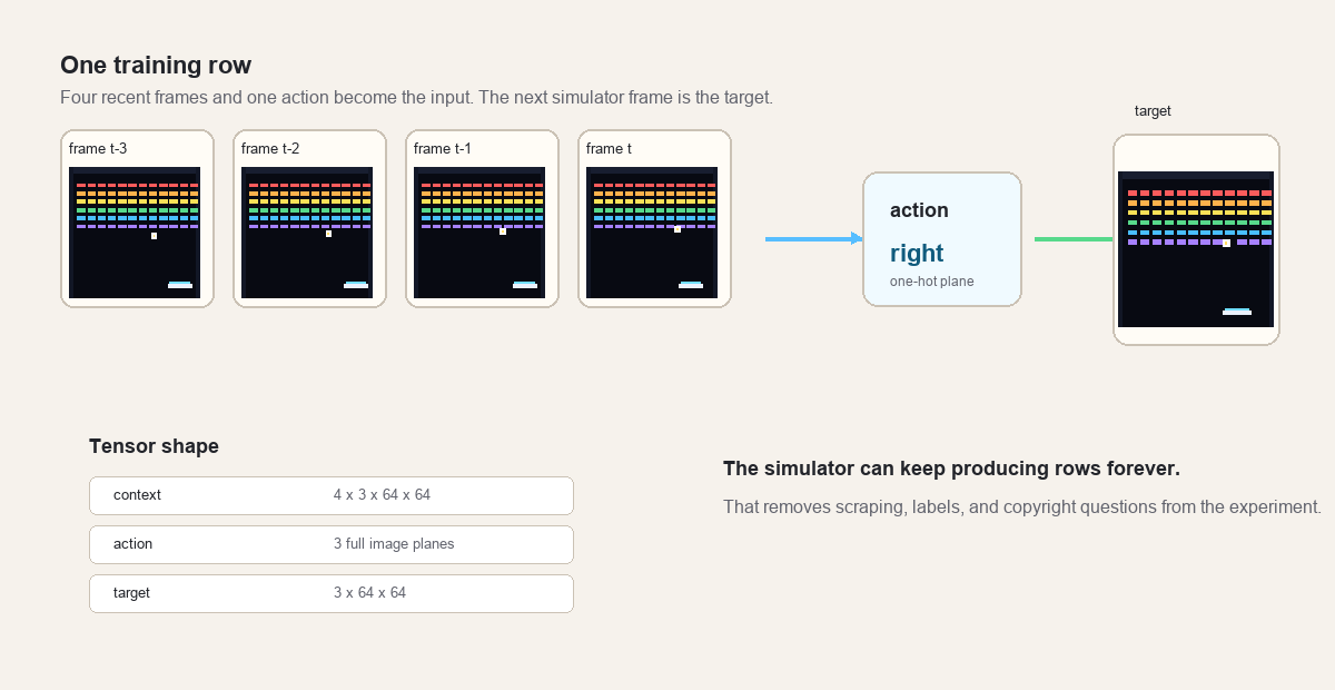
The action is not passed as a single scalar floating beside the image. It is expanded into three full image planes, one plane for each possible action. If the action is right, the right plane is full of ones and the other two are zeros.

This keeps the model fully convolutional. Every pixel sees the same action signal.

The row shapes are:

context: 4 frames * 3 channels * 64 * 64
action:  3 action planes * 64 * 64
target:  3 channels * 64 * 64

I like this part because there is no fixed dataset to babysit. The training loop asks the simulator for another batch. If the model needs more examples, the code makes more.

The tiny world model

Here, the world model is just a next-frame predictor. It is not a planner. It is not a game engine.

It learns this conditional distribution:

next frame given recent frames and action

The word “conditional” is doing real work. A video model that only sees frames can guess where the ball is already going. A game model also has to react to a new input. The same four frames can lead to different next frames if the player presses left, right, or nothing.

The model also stays at pixel level. No latent state. No recurrent hidden memory. No learned object list. I want those later, but the first experiment is easier to debug when the full chain is visible:

pixels in -> tiny model -> pixels out

The failures are visible too. If the model blurs the ball, invents a brick, or forgets the paddle, the canvas shows it.

Denoising the next frame

The model is trained as a denoiser.

Start with the real next frame from the simulator. Add Gaussian noise to it. Then ask the model to predict the clean frame from:

• the noisy target frame,
• the four context frames,
• the action planes,
• a sigma plane that says how much noise was added.

The clean target is often called x0 in diffusion code. Here x0 is not a latent or a hidden object. It is the clean next RGB frame.

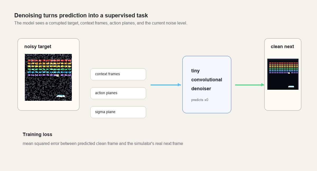
The model input has 19 channels:

Channels	Meaning
3	noisy target RGB frame
12	four RGB context frames
3	action planes for noop, left, right
1	sigma plane

The loss is mean squared error between the model output and the clean target frame.

Compared with a text-to-image diffusion system, this is tiny. There is no text encoder, classifier-free guidance, or large U-Net. The training shape is still recognizable: show the model a noisy thing, tell it the noise level, give it conditioning, and train it to predict the clean thing.

The denoiser

The browser model is a small convolutional network.

The default trained version uses width 96 and 14 residual blocks. It has about 2.4 million parameters and exports to a roughly 9.4 MB ONNX file. ONNX is a portable model format: PyTorch writes it, and a runtime in another environment can execute it.

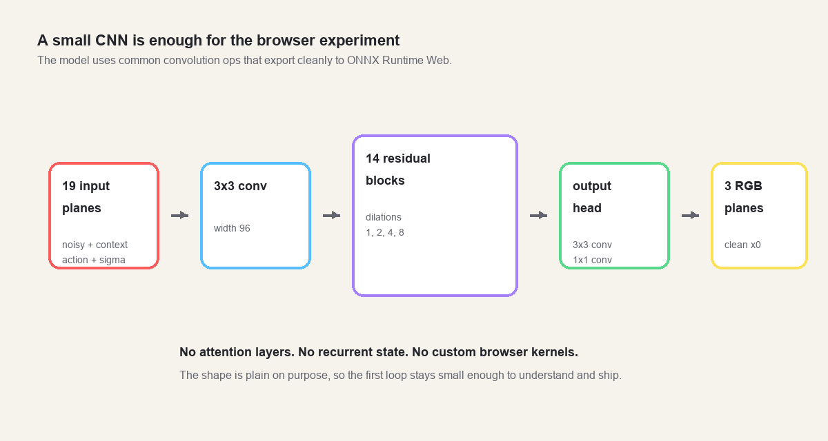
The residual blocks use dilated 3 by 3 convolutions. Dilation spreads the convolution taps apart, so a block can see a wider area without a larger kernel. The dilation pattern cycles through 1, 2, 4, 8.

Breakout has a lot of empty space. The ball, paddle, and bricks may be far apart, so the model needs enough receptive field to connect “the ball is moving down” with “the paddle is under it” and “the right key is pressed.”

The architecture works in the browser for a boring reason: it avoids exotic operators. Convolutions, SiLU activations, residual adds, and a final tanh are common ONNX operations. ONNX Runtime Web can run them with WebGPU when the browser supports it and WASM when it does not. In this demo, the WASM fallback uses ONNX Runtime’s hosted helper files from a CDN; those files could be self-hosted if the app needed to run without that dependency.

The training loop

The training loop fits on one screen.

For each step:

1. Ask the batched simulators for context frames, actions, and target frames.
2. Normalize frames from bytes into [-1, 1].
3. Sample a noise level sigma between 0.02 and 1.0.
4. Add noise to the target frame.
5. Build the 19-channel input tensor.
6. Run the model.
7. Compute mean squared error against the clean target.
8. Backpropagate, clip gradients, and update weights with AdamW.
9. Periodically save checkpoints and sample grids.

The sample grids matter because a scalar loss will lie to you by omission. A falling loss can still hide a model that blurs the ball, washes out bricks, or falls apart when its own predictions become the next input.

Evaluation rollouts make that failure easier to see. The script can run the real simulator beside the neural predictor and write a GIF. That comparison is stricter than one-step prediction because every neural mistake becomes part of the next context window.

Exporting to the browser

The exporter loads a PyTorch checkpoint, rebuilds the same TinyDenoiser, and writes one ONNX graph with a single input and output:

input: [1, 19, 64, 64]
pred:  [1, 3, 64, 64]

The browser loads the ONNX bytes and creates an ONNX Runtime Web session:

execution providers: webgpu, wasm

At inference time, the TypeScript sampler does this:

1. Converts the recent context frames into normalized channel planes.
2. Converts the current action into three action planes.
3. Builds a geometric sigma schedule.
4. Runs the denoiser a few times.
5. Converts the final [-1, 1] RGB output back into bytes.

The demo slider controls how many denoising steps to run. More steps can make the dream layer more coherent, but every step is another browser inference call. The demo has to stay responsive.

The sampling bug

The first neural rollout was not playable.

The model had learned a one-step denoising task, but the browser was asking it to start each next-frame sample from pure random noise. That makes sense for image generation. It is the wrong start for this game.

The next Breakout frame is usually very close to the latest Breakout frame. The bricks barely change. The paddle moves a few pixels. The ball moves a few pixels. Starting from pure noise throws away that structure, then asks a tiny model to rebuild the whole game state in a few browser steps.

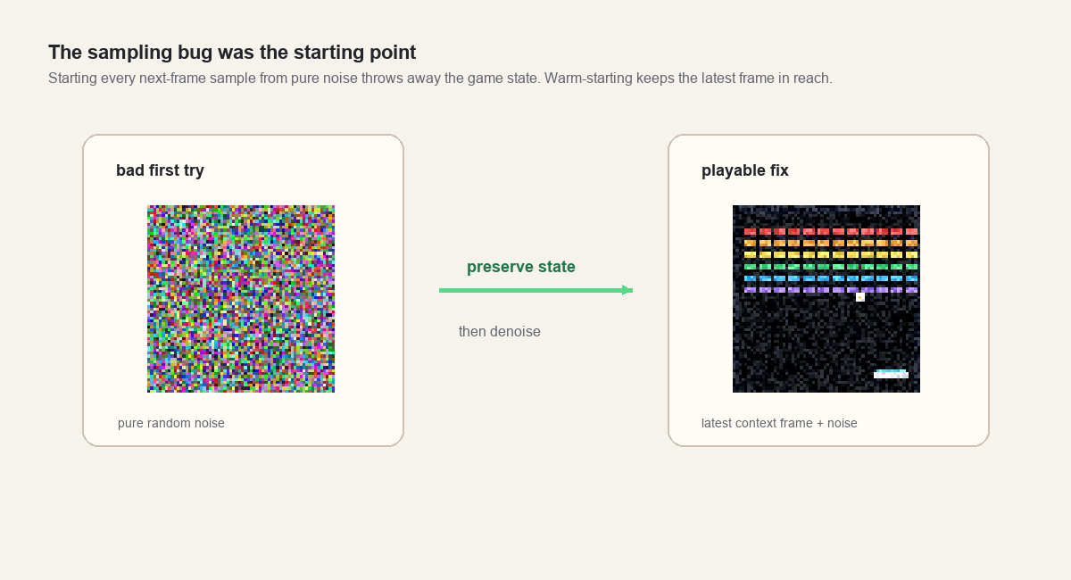
The fix was simple:

current = latest context frame + noise

Then the browser runs the denoising schedule from that warm start.

This changed the role of diffusion in the demo. The model stopped trying to generate the next game frame from scratch. It repaired a noisy version of the current state into a plausible next state.

A tiny browser model is much better at that repair job.

Making neural mode playable

The second fix was about authority.

An autonomous neural rollout is fragile. If the model predicts the ball one pixel too far left, the next context contains that error. Then the next prediction is built on the wrong ball position. Soon the model is playing its own drifting game.

Autonomous rollout is useful for studying long-horizon consistency, but it feels bad as a browser demo. Controls lag. Score becomes unclear. Collisions stop matching what the player sees.

So the playable version keeps the simulator authoritative.

The real simulator still advances every frame. It still reads the keyboard. It still owns score, lives, ball velocity, paddle position, bricks, and collision events. The neural model runs beside it at a lower cadence, predicts a dream layer from recent real context, and returns when inference is done. The browser blends the most recent completed neural frame over the real frame.

The result is less pure than a fully learned environment, but more honest at this stage.

The demo lets the player feel what the tiny model has learned without pretending it has solved long-horizon game simulation. The model can shimmer, drift, and invent artifacts. The game can still be played.

How I would scale it

The tiny version makes the tradeoffs visible. Scaling it is not a matter of turning one knob.

I would start with messier data. The current dataset comes from a simple scripted policy. A stronger dataset would include missed balls, bad paddle moves, weird brick patterns, resets, and recovery states. A model trained only on tidy play is brittle the moment a person plays badly.

After that, I would stop predicting raw pixels. Pixels are fine at 64 by 64. At larger sizes, the model should work in a latent space and spend more of its capacity on game structure instead of RGB detail.

The model also needs memory. Four frames are enough for short motion, but not for longer state. A recurrent model, a small state-space model, or a learned latent state would let the system carry information forward instead of re-inferring everything from a short context window.

The training objective would have to change too. One-step prediction is a clean starter task, but a real rollout forces the model to live with its own mistakes. Scheduled sampling, consistency losses, or latent correction could teach that recovery behavior.

And the browser loop has to stay cheap. More denoising steps can make the dream layer cleaner, but every step costs another inference call. A distilled sampler or a model trained for fewer steps would matter more than making the network slightly bigger.

The small game is a good place to make those changes because the whole stack is visible: simulator, data row, denoiser, sampler, export, browser loop, and the moment it stops feeling playable.